Viterbi Training - Part 1 Generating Data
Hidden Markov models (HMMs) are workhorses in computational biology. An HMM is useful when you believe the data you are observing is being generated by a process that can be in one of several distinct unobserved "states". We can observe the data, but the states are hidden. The states have different characteristics and the data generated by the system in each states differs in some sense.
The use of an HMM implies certain assumptions. Typically, the states are assumed to have a Markov property. That is you can predict the future of the process based solely on its present state, independent of its history. We can say that the future is conditionally independent of the past, given the present state. A second common assumption is that given the state, the data elements are independent. That is, the data generated depends only on the state of the system, not the preceding data items. It's the states that have a Markov property, not the data. This second assumption is sometimes relaxed to make hybrid HMMs.
In the figure below, the x's are the states and the y's are the data. The data are independent of one another. The states exhibit a Markov property.
HMMs are used in many fields, anytime you need to recover a sequence of states that is not immediately observable, but the output data is. HMMs are used in areas as diverse as finance, cryptanalysis, speech recognition and generation, machine translation, sequence analysis, gene prediction etc. The classic reference on HMMs is from Rabiner. Another good reference for HMMs in biological sequence analysis is the Durbin et al. book Biological Sequence Analysis.
You might want to use an HMM when you observe data that looks like the data has regions that appear "different" is some way. Here's an example.

It looks like there might be two different regions of data, one bouncing around near values of three and a lower region. A histogram of the data shows that the data might have a bi-modal distribution composed of a mixture of two normal distributions.

This is actually fictitious data generated as an example. It consists of values generated from one of two normal distributions, each with its own mean and standard deviation. To generate this data, we used two different normal distributions, one with a mean of 0 and standard deviation of 1, and the other with mean 3 and standard deviation 1. The means differ by quite a bit so that the different states can be visually distinct. In HMM terms, these are called the emission parameters. When observing the data, we don't know from which state each data item was emitted. There is a probability that any data point could be emitted from either state.
To generate the data, we first choose a starting state, either state 0 or 1. We'll index our states and emissions starting at 0. From the chosen state, we emit a value sampled from a normal distribution with the state's mean and standard deviation.
From the current state we want to chose the next state. Suppose the process is in state 0 at some point, i. At the next point, i+1, it could be in either state 0 or 1. The next state is chosen probabilistically. From each state there is a probability of staying in the same state or jumping to another state. In practical terms, we represent these transition probabilities as a transition matrix. If the set of transition and emission probabilities do not change within the sequence, the data is said to represent a stationary Markov process.
This Python routine will generate a set of sequences given a matrix of normal emission probabilities and a transition matrix.
This process of generating data in this way is an example of a generative model. You might think of this model as a machine that operates in two modes. One that spits out numbers with a mean of 0 and one that spits the numbers out with a mean of 3.
A full program for generating data Markov data from normal distributions along with some sample data output is available here. The program reads the number of states, and emission and transition parameters from a json file and outputs data sequences and states. Here is an example json file.
Download the code.
Next up - the Viterbi algorithm.
The use of an HMM implies certain assumptions. Typically, the states are assumed to have a Markov property. That is you can predict the future of the process based solely on its present state, independent of its history. We can say that the future is conditionally independent of the past, given the present state. A second common assumption is that given the state, the data elements are independent. That is, the data generated depends only on the state of the system, not the preceding data items. It's the states that have a Markov property, not the data. This second assumption is sometimes relaxed to make hybrid HMMs.
In the figure below, the x's are the states and the y's are the data. The data are independent of one another. The states exhibit a Markov property.
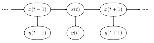 |
| By Qef - Own work by uploader, layout copied from bitmap Hmm temporal bayesian net.png, Public Domain, Link |
HMMs are used in many fields, anytime you need to recover a sequence of states that is not immediately observable, but the output data is. HMMs are used in areas as diverse as finance, cryptanalysis, speech recognition and generation, machine translation, sequence analysis, gene prediction etc. The classic reference on HMMs is from Rabiner. Another good reference for HMMs in biological sequence analysis is the Durbin et al. book Biological Sequence Analysis.
You might want to use an HMM when you observe data that looks like the data has regions that appear "different" is some way. Here's an example.


This is actually fictitious data generated as an example. It consists of values generated from one of two normal distributions, each with its own mean and standard deviation. To generate this data, we used two different normal distributions, one with a mean of 0 and standard deviation of 1, and the other with mean 3 and standard deviation 1. The means differ by quite a bit so that the different states can be visually distinct. In HMM terms, these are called the emission parameters. When observing the data, we don't know from which state each data item was emitted. There is a probability that any data point could be emitted from either state.
To generate the data, we first choose a starting state, either state 0 or 1. We'll index our states and emissions starting at 0. From the chosen state, we emit a value sampled from a normal distribution with the state's mean and standard deviation.
From the current state we want to chose the next state. Suppose the process is in state 0 at some point, i. At the next point, i+1, it could be in either state 0 or 1. The next state is chosen probabilistically. From each state there is a probability of staying in the same state or jumping to another state. In practical terms, we represent these transition probabilities as a transition matrix. If the set of transition and emission probabilities do not change within the sequence, the data is said to represent a stationary Markov process.
This Python routine will generate a set of sequences given a matrix of normal emission probabilities and a transition matrix.
"""
GenerateSequences - generate a set of sequences drawn from normal distributions
arguments: em - an n x 2 numpy array or list of lists of emission parameters. In each row
                the first element is the mean of a normal distribution and the second
                is the standard deviation.
           tr - transition matrix.
           num - how many sequences to generate
           seq_len - the length of each sequence.
requires: Each row of tr must sum to 1. em must be n x 2, tr must be n x n. n is the number of states.
returns: seqs - a list of sequences. Each sequence is a numpy array of floats.
         states - a list of the  generated states for each sequence.
"""
def GenerateSequences(em, tr, num, seq_len):
    num_states = em.shape[0]
    seqs = []
    states = []
    for n in range(num):
        s = []
        sts = []
        # select a starting state
        state = np.random.choice(num_states, size=1, p=tr[0, :])[0]
        for _ in range(seq_len):
            sts.append(state+1)
            # sample a value from the current state
            s.append(np.random.normal(em[state, 0], em[state, 1]))
            # get the next state based on the ansition matrix.
            state = np.random.choice(num_states, size=1, p=tr[state, :])[0]
        seqs.append(np.array(s))
        states.append(np.array(sts))

    return seqs, states
This process of generating data in this way is an example of a generative model. You might think of this model as a machine that operates in two modes. One that spits out numbers with a mean of 0 and one that spits the numbers out with a mean of 3.
A full program for generating data Markov data from normal distributions along with some sample data output is available here. The program reads the number of states, and emission and transition parameters from a json file and outputs data sequences and states. Here is an example json file.
{
    "states": 2,

    "transition": [
    {
        "from": 0,
        "to":   0,
        "prob": 0.9
    },
    {
        "from": 0,
        "to":   1,
        "prob": 0.1
    },
    {
        "from": 1,
        "to":   1,
        "prob": 0.95
    },
    {
        "from": 1,
        "to":   0,
        "prob": 0.05
    }
    ],

    "emission": [
    {
        "state": 0,
        "mean": 0,
        "std": 1
    },
    {
        "state": 1,
        "mean": 3,
        "std": 1
    }
    ]
}
Download the code.
Next up - the Viterbi algorithm.


Comments
Post a Comment