Mixed Models Part 2

 In a previous post, we looked at four different linear models for a collection of data where besides x and y values, the data was qualifies by an additional factor called a Group.

In those models, we either assumed that the difference in groups had no effect on the model, models 1 and 2, or that the groups were independent, and we could estimate their effects on slope and intercept individually. A compromise between these two approaches is the mixed-effect model, sometimes called a multilevel linear model or a random effects model. The difference is that the groups are assumed to be a random sample from a larger population of groups measuring the same kinds of data. In other words, are the groups we see all the groups we will see or is the data a sample from the world of possible groups?

A Linear Model

The simplest mixed model is similar to model 2 from the previous post. In this model we expect the Group value to affect the intercept of the linear model.

 \[\begin{array}{l}{y_i} = {\beta _{0j}} + {\beta _1}x + {\varepsilon _i}\\y \sim N({\beta _{0j}} + {\beta _1}x,\sigma _x^2)\\{\beta _{0j}} \sim N({\mu _{{\beta _0}}},\sigma _{{\beta _0}}^2)\end{array}\]

The difference from the similar linear model is the term ${\beta _{0j}} \sim N({\mu _{{\beta _0}}},\sigma _{{\beta _0}}^2)$. Here, rather than assuming ${\beta _0}$ is constant, we are assuming that the Group level indicators come from a normal, but with unknown parameters, distribution. Mixed effects models use a maximum likelihood method to estimate the coefficients and the variance of the coefficient.  

In this model, x is called a fixed effect and Group is called a random effect. However, in statistical literature the terms have fluid meanings. (See https://stats.stackexchange.com/questions/4700/what-is-the-difference-between-fixed-effect-random-effect-and-mixed-effect-mode and https://statmodeling.stat.columbia.edu/2005/01/25/why_i_dont_use/ for different definitions of fixed and random effects.) For our purposes, anything inside the parenthesis in an R formula is a random effect. Group as a random effect, indicates that we want to allow Group to influence the intercept of the model.

 In R terms:

> library(lmerTest)
> library(rsq)
> lmm1 <- lmer(y ~ x + (1 | Group), data = df_test, REML = FALSE, control = lmerControl(optimizer = "Nelder_Mead"))
> rsq(lmm1) # r-squared
$model
[1] 0.9431799

$fixed
[1] 0.9201095

$random
[1] 0.02307045

> 

effect	group	term	estimate	std.error	statistic	df	p.value	Significance
fixed	NA	(Intercept)	0.425990318	0.049594947	8.589389522	32.91957856	6.44E-10	***
fixed	NA	x	0.047049294	0.000430711	109.2364163	999.9529208	0	***
ran_pars	Group	sd__(Intercept)	0.182703789	NA	NA	NA	NA
ran_pars	Residual	sd__Observation	0.262164699	NA	NA	NA	NA

The table shows estimates for the fixed effects, intercept and slope. For the random effects we are provided with estimates of the standard deviation for Group and the model, i.e. $\sigma _{{\beta _0}}^2$ and $\sigma _x^2$. The standard deviation of the intercept shows the variability in the intercept across groups.

 We can also obtain estimates of the intercept and the random effect of each group on the intercept. The coefficients are calculated as the fixed effect for intercept + the random effect.

> write_mixed_model_coefs(lmm1, 'models/lmm1_coef.csv')

intercept	x	Group	ranef_intercept
0.365138253	0.047049294	1	-0.060852065
0.297419984	0.047049294	2	-0.128570334
0.430316754	0.047049294	3	0.004326436
0.429700924	0.047049294	4	0.003710606
0.659971258	0.047049294	5	0.23398094
0.793991226	0.047049294	6	0.368000908
0.395911819	0.047049294	7	-0.030078499
0.611620526	0.047049294	8	0.185630208
0.19373114	0.047049294	9	-0.232259178
0.353416766	0.047049294	10	-0.072573552
0.209006939	0.047049294	11	-0.216983379
0.641626397	0.047049294	12	0.215636079
0.487901608	0.047049294	13	0.06191129
0.091383548	0.047049294	14	-0.33460677
0.463582185	0.047049294	15	0.037591867
0.417185297	0.047049294	16	-0.008805021
0.256496571	0.047049294	17	-0.169493747
0.364360738	0.047049294	18	-0.06162958
0.40266712	0.047049294	19	-0.023323198
0.436768508	0.047049294	20	0.01077819
0.643599117	0.047049294	21	0.217608799

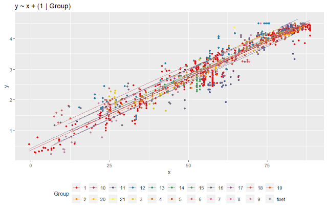
This plot appears similar to the plot from lmm3 from the previos post., but the shift in intercept is slightly less.  The "fixef" line shows the fixed effect intercept and slope.

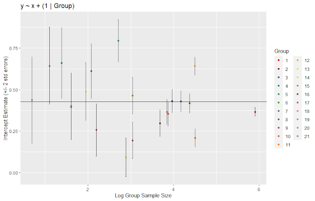
We can use the estimates and the standard error of the random effects to examine the effect of size. The plot shows the intercept estimates and +/- 2 standard errors. The horizontal line is the fixed effect estimate of the intercept. From the plot below, we see that labs with a small number of observations have larger standard errors. Near log(size) = 4 (about 55 observations) the standard errors are reduced, and the estimates are closer to the fixed effect estimate of the intercept.

Varying Slope and Intercept

As with the regression models, we can allow the slope to vary with Group. We will try this in two different ways. We can model variation is the slope as independent of variation in the intercept or as correlated with intercept as in a linear equation.

\[\begin{array}{l}{y_i} = {\beta _{0j}} + {\beta _{1j}}x + {\varepsilon _i}\\y \sim N({\beta _{0j}} + {\beta _{1j}}x,\sigma _x^2)\\{\beta _{0j}} \sim N({\mu _{{\beta _0}}},\sigma _{{\beta _0}}^2)\,\,{\beta _{1j}} \sim N({\mu _{{\beta _1}}},\sigma _{{\beta _1}}^2)\end{array}\]

In R,

> lmm2 <- lmer(y ~ x + (1 | Group) + (0 + x | Group), data = df_test, 
    REML = FALSE, 
    control = lmerControl(optimizer = "bobyqa"))
> rsq(lmm2)
$model
[1] 0.9454617

$fixed
[1] 0.9202339

$random
[1] 0.02522783

> 

effect	group	term	estimate	std.error	statistic	df	p.value	Significance
fixed	NA	(Intercept)	0.441912771	0.056084539	7.879404526	20.52537169	1.23E-07	***
fixed	NA	x	0.046776353	0.000627214	74.5780174	6.799725224	3.68E-11	***
ran_pars	Group	sd__(Intercept)	0.198195525	NA	NA	NA	NA
ran_pars	Group.1	sd__x	0.001170298	NA	NA	NA	NA
ran_pars	Residual	sd__Observation	0.260799199	NA	NA	NA	NA

In this case, there are standard deviations for random effects for slope and intercept.  We see that the random effect of Group on x covers only a very small proportion of the total variance while the effect of Group on the intercept covers more. 

We can plot the individual labs.

 

In this model, we only see small changes in the slopes.

Finally, we can model the effect of Group on both the slope and intercept.

\[\begin{array}{l}{y_i} = {\beta _{0j}} + {\beta _{1j}}x + {\varepsilon _i}\\y \sim N({\beta _{0j}} + {\beta _{1j}}x,\sigma _x^2)\\\left( {\begin{array}{*{20}{c}}{{\beta _{0j}}}\\{{\beta _{1j}}}\end{array}} \right) \sim N\left( {\begin{array}{*{20}{c}}{\left( {\begin{array}{*{20}{c}}{{\mu _{{\beta _0}}}}\\{{\mu _{{\beta _1}}}}\end{array}} \right)}&{\left( {\begin{array}{*{20}{c}}{\sigma _{{\beta _0}}^2}&{\rho {\sigma _{{\beta _0}}}{\sigma _{{\beta _1}}}}\\{\rho {\sigma _{{\beta _0}}}{\sigma _{{\beta _1}}}}&{\sigma _{{\beta _1}}^2}\end{array}} \right)}\end{array}} \right)\end{array}\]

> lmm3 <- lmer(y ~ x + (1 + x | Group), data = df_test, 
    REML = TRUE, 
    control = lmerControl(optimizer = "Nelder_Mead"))
> rsq(lmm3)
$model
[1] 0.9472098

$fixed
[1] 0.9208767

$random
[1] 0.02633312

> 

effect	group	term	estimate	std.error	statistic	df	p.value	Significance
fixed	NA	(Intercept)	0.436631488	0.082690437	5.280314164	16.73261814	6.45E-05	***
fixed	NA	x	0.046688799	0.00078598	59.40201396	14.9205669	3.85E-19	***
ran_pars	Group	sd__(Intercept)	0.334591939	NA	NA	NA	NA
ran_pars	Group	cor__(Intercept).x	-1	NA	NA	NA	NA
ran_pars	Group	sd__x	0.002807165	NA	NA	NA	NA
ran_pars	Residual	sd__Observation	0.259399193	NA	NA	NA	NA

Again, the small standard deviation of the random effect on x indicates that this effect covers only a small proportion of the total variance (0.07%). 

The plot shows more variation than the previous one, but much less than the similar regression model.

The plot below shows the random effects for intercept and x along with +/- their standard deviations.

Testing the Null Hypothesis

We have three nested mixed models:

\[\begin{array}{l}lmm1:y \sim N({\beta _{0j}} + {\beta _1}x,\sigma _x^2);{\beta _{0j}} \sim N({\mu _{{\beta _0}}},\sigma _{{\beta _0}}^2)\\lmm2:y \sim N({\beta _{0j}} + {\beta _{1j}}x,\sigma _x^2);{\beta _{0j}} \sim N({\mu _{{\beta _0}}},\sigma _{{\beta _0}}^2);{\beta _{0j}} \sim N({\mu _{{\beta _1}}},\sigma _{{\beta _1}}^2)\\lmm3:y \sim N({\beta _{0j}} + {\beta _{1j}}x,\sigma _x^2);\left( {\begin{array}{*{20}{c}}{{\beta _{0j}}}\\{{\beta _{1j}}}\end{array}} \right) \sim N\left( {\begin{array}{*{20}{c}}{\left( {\begin{array}{*{20}{c}}{{\mu _{{\beta _0}}}}\\{{\mu _{{\beta _1}}}}\end{array}} \right)}&{\left( {\begin{array}{*{20}{c}}{\sigma _{{\beta _0}}^2}&{\rho {\sigma _{{\beta _0}}}{\sigma _{{\beta _{01}}}}}\\{\rho {\sigma _{{\beta _0}}}{\sigma _{{\beta _{01}}}}}&{\sigma _{{\beta _1}}^2}\end{array}} \right)}\end{array}} \right)\end{array}\]

In R terms,

lmm1: y ~ x + (1 | Group)

lmm2: y ~ x + (1 | Group) + (0 + x |Group)

lmm3: y ~ x + (1 + x| Group)

As before, we can perform use anova to test the hypothesis that simpler models are better. 

> anova(lmm1, lmm2, lmm3)
Data: df_test
Models:
lmm1: y ~ x + (1 | Group)
lmm2: y ~ x + (1 | Group) + (0 + x | Group)
lmm3: y ~ x + (1 + x | Group)
     npar    AIC    BIC   logLik deviance  Chisq Df Pr(>Chisq)    
lmm1    4 220.04 239.67 -106.021   212.04                         
lmm2    5 220.94 245.48 -105.470   210.94  1.101  1      0.294    
lmm3    6 200.45 229.90  -94.225   188.45 22.491  1  2.112e-06 ***
---
Signif. codes:  0 ‘***’ 0.001 ‘**’ 0.01 ‘*’ 0.05 ‘.’ 0.1 ‘ ’ 1

We see that we can reject the null hypothesis, at least for lmm3, given the small p-values. In addition, AIC, BIC, and the loglikelihood for lmm3 show that the more complex model is an improvement over the simpler models.

Code for these models can be found on GitHub.