Delta Subvariant AY.4.2

IN OCTOBER 2019, just a few months before the novel coronavirus swept the world, Johns Hopkins University released its first Global Heath Security Index, a comprehensive analysis of countries that were best prepared to handle an epidemic or pandemic. The United States ranked first overall, and first in four of the six categories—prevention, early detection and reporting, sufficient and robust health system, and compliance with international norms. That sounded right. America was, after all, the country with most of the world’s best pharmaceutical companies, research universities, laboratories, and health institutes. But by March 2020, these advantages seemed like a cruel joke, as Covid-19 tore across the United States and the federal government mounted a delayed, weak, and erratic response. By July, with less than 5% of the world’s population, the country had over 25% of the world’s cumulative confirmed cases. Per capita daily death rates in the United States were ten times higher than in Europe. Was this the new face of American exceptionalism?

― Fareed Zakaria, Ten Lessons for a Post-Pandemic World 

It's a complicated scientific problem to update the sequence classification system, entirely maintained by academics," he told Newsweek. "And usually that kind of thing happens on a time scale of years, whereas now the whole world expects daily updates, and occasionally things break in a kind of obvious way like where the number of states changes day to day.

~ Jeffrey Barrett Wellcome Sanger Institute

The Delta variant (B.1.617.2) of SARS-CoV-2 continues to evolve. There have been enough changes to the designated variants that Pango has started classifying subvariants. For example subvariants of Delta are labeled AY.1 to AY.28.  The subvariant AY.4.3 has been reported to have increased transmissibility over the original Delta variant. Today, I will look at its growth in UK where its frequency has been seen to be expand.

First, I would like to look at the variants of concern in the USA and United Kingdom.  On Nov. 1, 2021, I downloaded 4,771,163 SARS-CoV-2 records from GISAID. Here are plots of the occurrences of the variants of concern in the two countries.

The linear growth of the Delta variant on the log scale shows that this variant is experiencing exponential growth in the number of cases in the data. The drop off in mid-October is likely caused by a lag in the submission of sequences in recent weeks. The R code for these graphs can be found here.

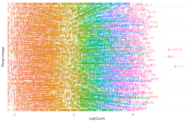
The number of subvariants of is becoming bewildering large. This messy plot shows the large collection of subvariants.

The R code for this plot:

#' plot_pango_lineages - produce a messy plot of Pango lineages and their log counts.
#'
#' @param meta_data A GISAID variant table read by read.csv.
#'
#' @return a dataframe with columns Variant, Pango.lineage, log_count, and y_random.
#' y_random is the position of the vraiant label on the y axis.
#' 
plot_pango_lineages <- function(meta_data) {
  # from https://stackoverflow.com/questions/66807383/best-way-to-visualize-counts-for-very-large-number-of-variables-with-ggplot
  
  library(dplyr)
  library(ggplot2)
  library(ggrepel)
  
  # count variants 
  df2 <- meta_data %>% 
    select(Variant, Pango.lineage) %>% 
    group_by(Variant, Pango.lineage) %>% 
    count() %>%
    mutate(n = log(n)) %>%
    rename(log_count = n)
  
  # put them at random on y axis
  df2$y_random <- c(runif(nrow(df2), min = -1, max = 1))
  
  # plot
  p <- 
    df2 %>% 
    ggplot(aes(x = log_count, y = y_random, label = Pango.lineage, color = as.factor(log_count))) +
    geom_text_repel(max.overlaps = 500) +
    theme_minimal() +
    theme(legend.position = "None",
          axis.ticks.y = element_blank(),
          axis.text.y = element_blank()) +  
    labs(x = "Log(Count)",
         y = "Pango.lineage")
  
  print(p)
    
  return(df2)
}

AY.4.2

The AY.4.2 subvariant of the Delta variant has been expanding in the United Kingdom since July 2021.  It contains mutations A222V and Y145H in its spike protein,. It has been suggested that AY.4.2 might be 10-15% more transmissible than the original Delta variant. 

In addition to the two mutations listed above AY.4.2 typically has a number of differences from the reference sequence; N_G215C, NSP3_A1711V, Spike_T95I,N_D63G, N_R203M, NSP12_G671S, Spike_G142D, NS3_S26L, Spike_P681R, Spike_R158del, NSP3_P1228L, NS7a_V82A, NSP3_A488S, Spike_F157del, N_S202I, NSP4_T492I ,NSP14_A394V, Spike_T19R, NS7a_T120I, Spike_A222V, N_D377Y, M_I82T, Spike_D950N, NS7b_T40I, NSP13_P77L, NSP4_V94A, Spike_E156G, NSP3_P1469S, Spike_T478K, Spike_Y145H, NSP6_T77A, Spike_V36F, NSP12_P323L, NSP12_F694Y, Spike_D614G, NSP4_V167L, Spike_L452R.

We can filter the Pango lineages to see the growth of this subvariation.

> df_uk_voc_pango <- pango_lineages(meta_data, country = 'United Kingdom', VOC_only = TRUE)
> df_uk_AY_4_2 <- df_uk_voc_pango %>% filter(Pango.lineage == 'AY.4.2')}
> ggplot(df_uk_AY_4_2) + geom_point(aes(x = Collection.date, y = log(Count))) + ggtitle('UK AY.4.2 2021-11-01')

Again we can see linear growt in the log scale indicating an exponential increase in the counts.

Here's the code to select the Pango lineages.

#' pango_lineages Select records containing Pango lineages for a country and host.
#'
#' @param meta_data A GISAID variant table read by read.csv.
#' @param host      A string indicating host species.
#' @param country   Country of interest. If NULL, all countrys are included.
#' @param VOC_only  A logical. Should only variants of concern be included
#'
#' @return
#' @export
#'
#' @examples
pango_lineages <- function(meta_data,
                           host = "Human", 
                           country = "USA", 
                           VOC_only = FALSE) {
  library(tidyverse)
  
  # Select columns and split location. Select VOC.
  df <- meta_data %>% 
    filter(host == {{ host }}) %>%
    select(Collection.date, Location, Variant, Pango.lineage) %>% 
    separate(Location, c("Region", "Country", "State"), sep = "\\s*/\\s*", extra = "drop", fill = "right") %>%
    select(-c("Region", "State")) %>%
    mutate(Collection.date = as.Date(Collection.date, format = "%Y-%m-%d")) %>%
    filter(! is.na(Collection.date)) %>%
    separate(Variant, c("V", "Name"), extra = "drop", fill = "right") %>%
    unite(Variant, V:Name, sep = " ", remove = TRUE) %>%
    mutate(Variant = as.factor(Variant))
  
  # Remove non VOC is need to.
  if(VOC_only) {
    df <- df %>% filter(Variant != '')
  }
  
  # Filter by country and lineages
  # Count by date and lineage
  if(! is.null(country)) {
    df <- df %>%
      filter(Country == {{ country }})
  }

  df2 <- df %>%
    group_by(Collection.date, Pango.lineage) %>% 
    count() %>%
    rename(Count = n)
  
  return(df2)
}

I can't show a similar plot for the US. Although it has been reported that AY.4.2 has been detected in 32 US states, the GISAID database only shows 10 sequences for the US compared to 25,161 for the UK. We have see that it takes several weeks for the sequences to go from collection to the data. Real time tracking of viral sequences would be ideal, but unlikely right now due the constrains on collection and sequencing technology.