A Slightly Better Neural Net Regression
I hesitate to call this deep learning. Anything running on a PC isn't all that deep.
We looked at fitting this data using a neural net previously This time we will add a new set of data, global mean CO2 levels. In addition, instead of simple linear layers, we will use a fully recurrent neural network (RNN) as an initial layer.
The data we will analyze is from this post. It represents Temperature Anomaly estimates for the period 1850 to 2021 from the NASA Global Climate Change site. We have seen this data before: here, here, and here.
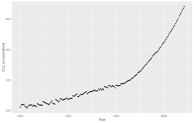
In addition, we will add a second source of data - the global mean CO2 concentration from 1850 through 2021 from Our World in Data. There are missing values in the downloaded data. They are replaced with linear interpolation using na.approx from the R zoo package.
CO2_conc <- atmospheric_data %>%
    filter(Entity == 'World' & Year >= 1850 & Year <= 2021) %>%
    select(Year, CO2.concentrations) %>%
    na.approx() %>%
    as.data.frame()
A Simple RNN
We will use the PyTorch library to build the neural net. To get started, here's our simple RNN.class RNet(torch.nn.Module): def __init__(self, hidden_size = 10, num_layers = 1): super(RNet, self).__init__() self.rnn1 = torch.nn.RNN(input_size = 1, hidden_size = hidden_size, num_layers = num_layers) self.linear1 = torch.nn.Linear(hidden_size, 2) self.leaky_rlu = torch.nn.LeakyReLU() def forward(self, x): x = x.unsqueeze(dim = 1) x, _ = self.rnn1(x) x = self.leaky_rlu(x) x = self.linear1(x) return x.squeeze(dim = 1) # RNN
Training
python rnn_regression.py -e 2000 -w 10 -n 30 -b 64 -p 5 -l 1 ../data/temperature.csv ../data/CO2_conc_1850.csv
# construct the model
    net = RNet(hidden_size = hidden_size, num_layers = num_layers)

    optimizer = torch.optim.Adam(net.parameters(), lr = lr)
    loss_func = torch.nn.SmoothL1Loss()  # Smooth loss - less ensitive to outliers

    # set up data for loading
    dataset = Data.TensorDataset(x, y)
    loader = Data.DataLoader(
        dataset = dataset,
        batch_size = batch_size,
        shuffle = True,
        num_workers = workers,)
hidden_size is the size of the RNN hidden layer. Data is torch.utils.data. lr is the learning rate (0.01). We use the Adam optimizer and a smoothed L1 loss function. We will use workers tasks to process each epoch.
The training loop calculates the loss and updates the weights. It saves the model which has the minimum loss seen so far.
    # start training
    best_model = None
    min_loss = sys.maxsize
    for epoch in range(epochs):
        for step, (batch_x, batch_y) in enumerate(loader): # for each training step

            prediction = net(batch_x)

            loss = loss_func(prediction, batch_y)
            print('epoch:', epoch, 'step:', step, 'loss:', loss.data.numpy())
            if loss.data.numpy() < min_loss:
                min_loss = loss.data.numpy()
                best_model = copy.deepcopy(net)

            optimizer.zero_grad()   # clear gradients for next train
            loss.backward()         # backpropagation, compute gradients
            optimizer.step()        # apply gradients
 # get a regression fit
    best_model.eval()
    prediction = best_model(x)
r2 = r2_score(y.data.numpy(), prediction.data.numpy()) # predict the future future_predict = best_model(torch.cat((x, x_predict)))[-predict_size:, :]
Prediction is hard, especially the future...
input_file1 = /mnt/d/Documents/analytic_garden/Torch/CO2/data/temperature.csv
input_file2 = /mnt/d/Documents/analytic_garden/Torch/CO2/data/CO2_conc_1850.csv
output_path = /mnt/d/Documents/analytic_garden/Torch/CO2/output2
predict_size = 5
batch_size = 64
epochs = 2000
learning_rate = 0.01
rnn_out1 = 20
rnn_out2 = 10
workers = 10
rand_seed = 1649438337
R^2 = 0.9552628273845742
Best model loss = 0.009633683


Comments
Post a Comment